3. Back End Module

Front-end process only possesses transient memory which is not enough to keep the entire motion trajectory in an optimal state. So we use the back-end technique to consider the long-term state estimation problem, updating its own state using the past information. The back-end is usually either a filtering framework (like EKF) or graph optimization (i.e. Bundle Adjustment ). Nowadays, graph optimization is much more popular benefiting from more powerful processors. The general idea of graph optimization is to express the SLAM problem as a graph structure.

Fig. 3.1 The overview structure of back-end module.

3.1. Nonlinear Least Square problem

For SLAM problems, a keyframe pose of the robot or a landmark position in the map is denoted as a node, while the observations and geometric model between keyframe-keyframe, keyframe-landmark, or landmark-landmark are denoted as the constraints that connected certain nodes. The front-end actually constructs the graph, and the back-end manages to adjust the vertices so as to satisfy the constraints of the edges.

Given a graph, graph optimization aims to find an optimal estimation of the nodes values which minimize the errors that determined by the constraints. Therefore, SLAM back-end is transformed to be a least squares minimization problem, which can be described by the following equation:

(3.1)\[\begin{split}\begin{align} \mathbf{F}(\mathbf{x}) & =\sum_{<i,j>\in{\mathcal{C}}}\mathbf{e}(\mathbf{x}_i,\mathbf{x}_j,\mathbf{z}_{ij})^{\intercal} \mathbf{\Omega}_{ij}\mathbf{e}(\mathbf{x}_i,\mathbf{x}_j,\mathbf{z}_{ij}) \\ & = \sum_{<i,j>\in{\mathcal{C}}}\underbrace{\mathbf{e}_{ij}(\mathbf{x})^{\intercal} \mathbf{\Omega}_{ij} \mathbf{e}_{ij}(\mathbf{x})}_{\mathbf{F}_{ij}} \mathbf{x}^* \\ & =\underset{\mathbf{x}}{\operatorname{argmin}}\mathbf{F}(\mathbf{x}) \end{align}\end{split}\]

where \(\mathcal{C}\) the system graph, \(\mathbf{x}_i\) vertex, is the robot pose, \(\mathbf{z}_{ij}\) edge, is the measurement, and \(\mathbf{\Omega}_{ij}\) is the information matrix of this error.

Usually the solution of incremental optimization is iteratively finding the gradient to keep updating the current variables \(\mathbf{x}\) from an initial guess \(\breve{x}\) to approximate the cost function \(\mathbf{F}(\mathbf{x})\), until convergence. Around \(\breve{\mathbf{x}}\) we execute first order Taylor expansion of \(\mathbf{F}(\mathbf{x})\):

(3.2)\[\begin{split}\begin{equation} \begin{split} \mathbf{F}(\mathbf{x}+\mathbf{\Delta x}) & = \sum_{<i,j>\in{\mathcal{C}}} \mathbf{F}_{ij}(\mathbf{x}+\mathbf{\Delta x}) \\ & \simeq \sum_{<i,j>\in{\mathcal{C}}} \left(\mathbf{e}_{ij}+\mathbf{J}_{ij} (\mathbf{x})\mathbf{\Delta x}\right)^\intercal \mathbf{\Omega}_{ij}\left(\mathbf{e}_{ij}+\mathbf{J}_{ij} (\mathbf{x})\mathbf{\Delta x}\right) \\ & = \sum_{<i,j>\in{\mathcal{C}}} \underbrace{\mathbf{e}_{ij}^\intercal \mathbf{\Omega}_{ij} \mathbf{e}_{ij}}_{c_{ij}} + 2\underbrace{\mathbf{e}_{ij}^\intercal \mathbf{\Omega}_{ij} \mathbf{J}_{ij}}_{b_{ij}}\mathbf{\Delta x} + \mathbf{\Delta x}^\intercal \underbrace{\mathbf{J}_{ij}^\intercal \mathbf{\Omega}_{ij} \mathbf{J}_{ij}}_{H_{ij}}\mathbf{\Delta x} \\ & = \mathbf{c} + 2\mathbf{b}^\intercal \mathbf{\Delta x} + \mathbf{H\Delta x}^\intercal \mathbf{H \Delta x} \end{split} \end{equation}\end{split}\]

To get the minimization of this equation, we need to set the derivative of \(\nabla \mathbf{F}|_\mathbf{\Delta x}=0\), thus we obtain a linear equation:

(3.3)\[\begin{equation} \mathbf{H\Delta x}^* = -\mathbf{b} \end{equation}\]

where \(\mathbf{H}\) is the information matrix of the system (Note that different from \(\mathbf{H}\), \(\mathbf{\Omega_{ij}}\) is the information matrix of the graph edges). By adding the increments \(\mathbf{\Delta x}^*\) to the initial guess \(\breve{\mathbf{x}}\), we obtain the solution:

(3.4)\[\begin{equation} \mathbf{x}^* = \breve{\mathbf{x}} + \mathbf{\Delta x}^*. \end{equation}\]

The above process is the classical Gauss-Newton method by iteratively calculating equation (3.3) and (3.4). To obtain \(\mathbf{\Delta x}\), \(\mathbf{H}\) must be reversible, i.e. positive definite. But the real \(\mathbf{J}^\intercal\mathbf{J}\) only possesses the property of semi-positive definite, leaving \(\mathbf{H}\) the possibility of singular matrix or ill-condition, thus making the optimization process non-convergent. Therefore, some trust region methods are utilized in real application, like Levenberg-Marquardt (LM) and Dog-Leg algorithm, to make the solution more robust. The LM algorithm uses a damping factor to Gauss-Newton to control the step size of the convergence. Instead of solving equation (3.3), LM solves a damped but robust version. Here we give a simplified form:

(3.5)\[\begin{equation}\label{equ.lm} (\mathbf{H}+\lambda\mathbf{I})\mathbf{\Delta x}^* = -\mathbf{b} \end{equation}\]

where \(\lambda\) is the damping factor to dynamically tackle non-linear surfaces.

However, it is noteworthy that the procedures described above are just general means assuming the space of the parameters \(\mathbf{x}\) is Euclidean. This case does not apply for issues like VSLAM thus might lead to sub-optimal results. So on the base of on-manifold optimization theory we choose to use \(\mathbf{\Delta x}\) as perturbations around current variable \(\breve{\mathbf{x}}\) which is small thus non-singular. We consider the underlying space as a manifold and define an operator \(\boxplus\) which maps the local variable \(\mathbf{\Delta x}\) in the Euclidean space to a variable on the manifold: \(\mathbf{x}^* \mapsto \mathbf{\breve{x}}\boxplus \mathbf{\Delta x}^*\).

The \(\boxplus\) operator uses the motion compounding representation method to apply the increment \(\mathbf{\Delta x}\) to \(\mathbf{x}\). So the Jacobian \(\mathbf{J}_{ij}\) becomes:

\[\begin{equation} \mathbf{J}_{ij} = \frac{\partial \mathbf{e}_{ij}\left(\breve{\mathbf{x}\boxplus \mathbf{\Delta x}}\right)}{\partial \mathbf{\Delta x}} | _{\mathbf{\Delta x}=\mathbf{0}}. \end{equation}\]

The change of parametrization does not change the structure of the Jacobian \(\mathbf{J}\) and Hessian \(\mathbf{H}\). Actually some off-the-shelf non-linear solvers like g2o and ceres-solver are able to provide tools for computing the Jacobians on the manifold space.

3.2. Bundle Adjustment

Based on equation of (1.2) introduced in section Structure Overview, we formulate the reprojection error function with 3D point \(\mathbf{p}\in{\mathbb{R}^3}\) as landmark \(\mathbf{y}\) and Lie-algebra \(\mathbf{\xi}\) to represent pose \(\mathbf{x}\):

(3.6)\[\begin{equation} \mathbf{e} = \mathbf{z} - h\left(\boldsymbol {\xi},\mathbf{p}\right). \end{equation}\]

To be more specific for VSLAM problems, according to equation (2.3) introduced in section Front End Module, we can formulate a least square function to minimize the error and find the optimal camera poses:

\[\begin{equation} \boldsymbol{\xi}^* = \underset{\boldsymbol {\xi}}{\operatorname{argmin}}\frac{1}{2}\sum_{i=1}^{n}||\mathbf{u}_i-\frac{1}{s_i}\mathbf{K}\text{exp}\boldsymbol{\xi}^{\wedge}\mathbf{P}_i||^2_2 \end{equation}\]

To make the VLSAM solution more consistent, we add the constraints of landmarks in addition to camera poses. So our task is to use numerical means to handle the nonlinear model \(h\left(\boldsymbol {\xi},\mathbf{p}\right)\) by calculating the incremental value \(\Delta\mathbf{x}\) iteratively. The variables remained to be optimized are:

\[\begin{equation} \mathbf{x} = \left[\boldsymbol {\xi}_1, \cdots, \boldsymbol {\xi}_m, \mathbf{p}_1, \cdots, \mathbf{p}_n \right]^\intercal \end{equation}\]

where \(\boldsymbol {\xi}\) is the pose and \(\mathbf{p}\) is the landmark location variable. So based on equation (3.2) we build the cost function

\[\begin{equation} \frac{1}{2} || \mathbf{F}(\mathbf{x}+\mathbf{\Delta x}) || ^2 \approx \frac{1}{2}\sum_{i=1}^{m} \sum_{j=1}^{n} || \mathbf{e}_{ij}+\mathbf{D}_{ij}\mathbf{\Delta \xi}_i + \mathbf{E}_{ij}\mathbf{\Delta p}_j || ^2 \end{equation}\]

where Jacobian matrix \(\mathbf{D}_{ij}\) is the partial derivative of the entire cost function for the current camera pose, whereas \(\mathbf{E}_{ij}\) the partial derivative of the function for the landmark positions. Here we skip the derivation of these two types of matrices. Together the Jacobian matrix \(\mathbf{J}\) can be separated into blocks \(\mathbf{J}=\left[\mathbf{D E}\right]\). Take Gauss-Newton method as example, the \(\mathbf{H}\) matrix becomes

(3.7)\[\begin{split}\begin{equation} \mathbf{H}=\mathbf{J}^\intercal\mathbf{J}=\begin{bmatrix} \mathbf{D}^\intercal\mathbf{D} & \mathbf{D}^\intercal\mathbf{E} \\ \mathbf{E}^\intercal\mathbf{D} & \mathbf{E}^\intercal\mathbf{E} \end{bmatrix} = =\begin{bmatrix} \mathbf{H}_{11} & \mathbf{H}_{12} \\ \mathbf{H}_{21} & \mathbf{H}_{22} \end{bmatrix} \end{equation}\end{split}\]

When it comes to numerically solving nonlinear least squares optimization issues, we can use the matrix decompositions like Cholesky or QR. Especially for large-scale problems, these methods play a crucial role in reducing complexity and improving realtime performance 1.

However, when we have considered all the optimization variables, this matrix has a large amount of dimensions. In VSLAM problems, one frame usually contains hundreds of features, which dramatically increases the scale of the linear equation. If we directly calculate the inverse of \(\mathbf{H}\), the computational complexity is \(\mathcal{O}(n^3)\) making the computing processor drain out. Luckily Hessian \(\mathbf{H}\) has a special structure that can be utilized by us to accelerate the optimization process.

3.3. Sliding Window and Marginalization

3.3.1. Theory

One of the advantages of graph based optimization is the sparse structure of Hessian matrix \(\mathbf{H}\) 2. Each error \(\mathbf{e}{ij}\) in the cost function only describes the observed landmark \(\mathbf{p}_j\) at the camera pose \(\boldsymbol{\xi}_i\), leaving the derivatives of the remaining variables 0. So the Jacobian matrix corresponding to this error term \(\mathbf{e}_{ij}\) is:

(3.8)\[\begin{equation} \mathbf{J}_{ij}(\mathbf{x})=\left(\mathbf{0}_{2\times 6}, \cdots \mathbf{0}_{2\times 6}, \frac{\partial \mathbf{e}_{ij}}{\partial \boldsymbol{\xi}_i }, \mathbf{0}_{2\times 6}, \cdots \mathbf{0}_{2\times 3}, \cdots \mathbf{0}_{2\times 3}, \frac{\partial \mathbf{e}_{ij}}{\partial \mathbf{p}_j }, \mathbf{0}_{2\times 3}, \cdots \mathbf{0}_{2\times 3} \right). \end{equation}\]

From equation (3.7), \(\mathbf{H}_{11}\) is only relevant to camera pose and \(\mathbf{H}_{22}\) replies only on landmarks. So when we span over all the \(i,j\), we find the sparsity property of Hessian \(\mathbf{H}\):

• \(\mathbf{H}_{11}\) and \(\mathbf{H}_{22}\) are always diagonal matrices.

• For \(\mathbf{H}_{12}\) and \(\mathbf{H}_{21}\), it depends on the specific observation data.

Suppose a simple example that there are two camera poses (\(C_1,C_2\)) and 6 landmarks (\(P_1,\cdots,P_6\)) with corresponding state variable \(\boldsymbol{\xi}_i,i=1,2\) and \(\mathbf{p}_j,j=1,\cdots,6\). So the sparsity illustration of the overall Jacobian matrix and the corresponding \(\mathbf{H}\) matrix is as shown in figure 2. In a more general sense with \(m\) camera poses and \(m\) landmarks, we usually have \(n\gg m\). With this structure a couple of methods can be implemented to use this sparsity advantage. One of the most effective means is Marginalization.

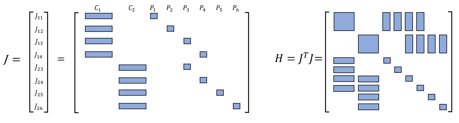
Fig. 3.2 The sparsity illustration of Jacobian matrix (Left) and that of \(\mathbf{H}\) matrix (Right).

3.3.2. Implementation

We incorporate marginalization to bound computational complexity. We selectively marginalize out IMU/INS states \(\mathbf{i}_k\) and features \(\lambda_l\) from the sliding window, meanwhile convert measurements corresponding to marginalized states into a prior.

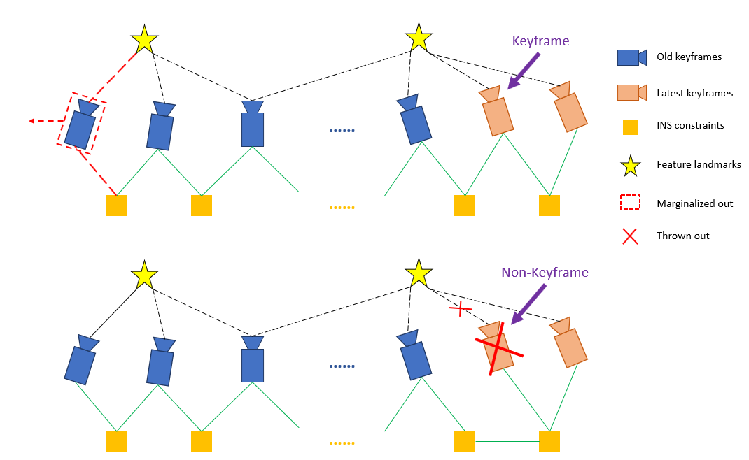
Fig. 3.3 Illustration of our marginalization strategy.

As shown in Fig. 3.3, when the second latest frame is a keyframe, it will stay in the window, and the oldest frame is marginalized out with its corresponding measurements. Otherwise, if the second latest frame is a non-keyframe, visual measurements are thrown away and only IMU/INS measurements that connect to this frame are kept.We do not marginalize out all measurements for non-keyframes in order to maintain sparsity of the system. The marginalization scheme aims to keep spatially separated keyframes in the window, which ensures sufficient parallax for feature triangulation.

The marginalization is carried out using the Schur complement 3. We construct a new prior factor based on all marginalized measurements related to the removed state Class MarginalizationFactor. New priors are continuously added into the existing priors.

The drawback of marginalization is that it results in the early fix of linearization points, which cause sub-optimal estimation results. However, we can tolerate this small drift for better speed accuracy trade-off (if we have INS assist, drifting errors will be reduced).

1

P. Krauthausen, A. Kipp, and F. Dellaert, “Exploiting locality in slam by nested dissection,” Georgia Institute of Technology, 2006.

2

L. Polok, V. Ila, M. Solony, P. Smrz, and P. Zemcik, “Incremental block cholesky factorization for nonlinear least squares in robotics.,” in Robotics: Science and Systems, 2013.

3

G. Sibley, L. Matthies, and G. Sukhatme, “Sliding window filter with application to planetary landing,” J. Field Robot., vol. 27, no. 5, pp. 587– 608, Sep. 2010.